Demo

If you want to test AutoPIA without buying a license, you can obtain a demo and try the software in your working environment with your images. This will allow you to understand the benefits of AutoPIA with respect to manual analysis. If you do not have working images, you can download some from the download page on CyberQual web site.

In order to test some features, mainly related with control charts, it is necessary to collect and insert lot of data, so to simulate the routine quality control of a radiological equipment. This can be very time-expensive. Therefore, AutoPIA has an integrated demo database, which contains data of almost one year of routine quality control and two images to simulate what happens during everyday activity.

In order to run the AutoPIA demo it is necessary to:

1. install the software (step-by-step procedure)
2. request a license (step-by-step procedure)
3. install license (step-by-step procedure)

When the AutoPIA instance is available on a PC, it is possible to play around with the program. The following steps describe a tour for discovering AutoPIA main features.

Step-by-step demo

Run AutoPIA: the analysis layout appears.

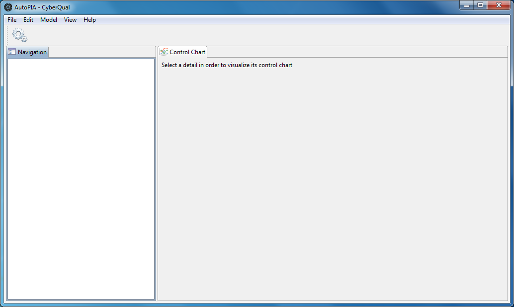
Switch to the control chart layout using the View | Result layout.

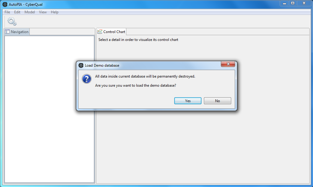
Load the demo database using the menu Model | Load demo DB. AutoPIA will ask you to confirm this operation, because it will delete all stored data; click on "Yes" to continue.

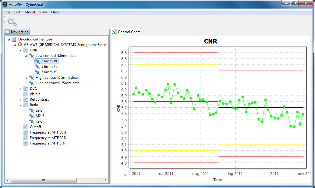
After a while a compressed tree will appears in the Navigation view; the hierarchy structure is composed by

• Medical centres
• Equipments
• IQIs
• Detail groups
• Details

Every leaf of the tree correspond to a control chart for an IQI of a certain detail of an equipment inside a medical centre. Selecting a leaf will show the corresponding control chart inside the Control Chart view.

Double clicking on the leaf opens a dialog where it is possible to edit the baseline definition: baselines can be divided in periods, each one defining the baseline value and the bounduaries.

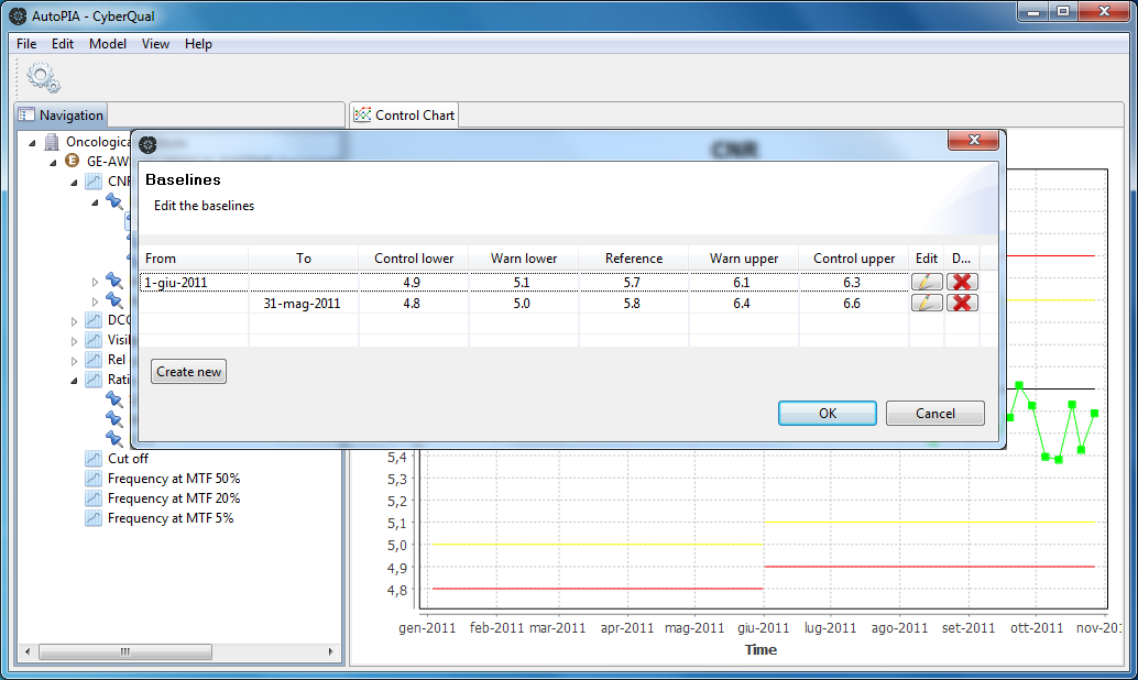
The dialog contains a table with one row for every period and the following columns:

• From:the date from which the values are valid (empty value means all values up to the To date)
• To:the date until when the values are valid (empty value means all values from the From date)
• Control lower:the lower bound of the control limit (delimited in red)
• Warn lower:the lower bound of the warninglimit (delimited in yellow)
• Reference:the baseline value (marked in black)
• Warn upper:the upper bound of the waninglimit (delimited in yellow)
• Control upper:the upper bound of the control limit (delimited in red)

There are also two icons in each row: one to edit the values of the baseline period (the row) and one to delete it. The "Create new" button below the table creates a new baseline period to be filled with meaningful values. Modifications takes effect only when the baseline dialog is closed with the "Ok" button.

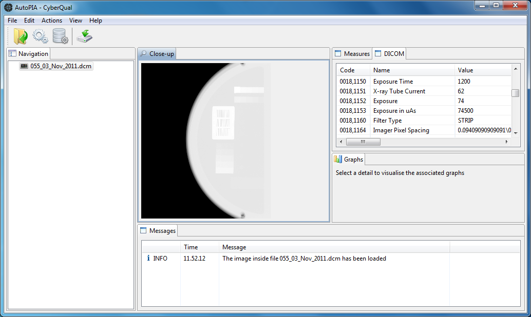
Let's simulate what happens during routine quality control: the personell produces an image produced by exposting the phantom in a specific equipment. Open the image: swith to the analysis workbench with menu View | Analysis layout.

Open the demo image 068_GE_Essential_25_Oct_2010.dcm (available in the download page on CyberQual web site) with menu File | Open. The file will appear inside the Navigation view. If you select it, the Close-up view will show the image and the DICOM view will enumerate all DICOM tags inclued inside the image.

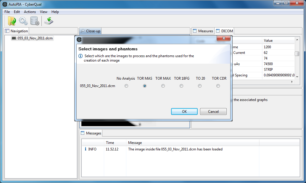
Start the analysis of the image with the menu Actions | Analyse. A dialog asks which is the phantom in the image: in this example it is a Leeds Test Objects TOR MAS. Select it and press "Ok".

When the analysis is completed the results are displayed: the image on the Navigation view becomes a tree, which is the hierarchical representation of the phantom. The root is the phantom itself (it has no IQIs), then there are some groups of details (e.g. for TOR MAS the Perpendicular high resolution grid, the low contrast circular detail, ...), and so on depending on the phantom layout.

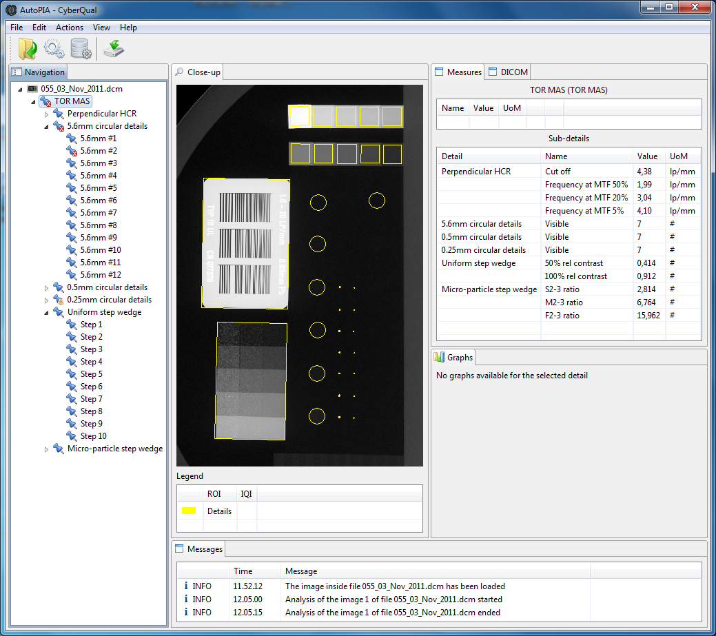
Every node is a detail group (set of details) or a single detail: both may have their own IQIs and physical properties. IQIs of the selected detail group or detail are listed inside the first table of the Measures view, while the second table lists the IQIs of the cchildren (if any). For example, select the "5.6mm circular details" node of the tree.

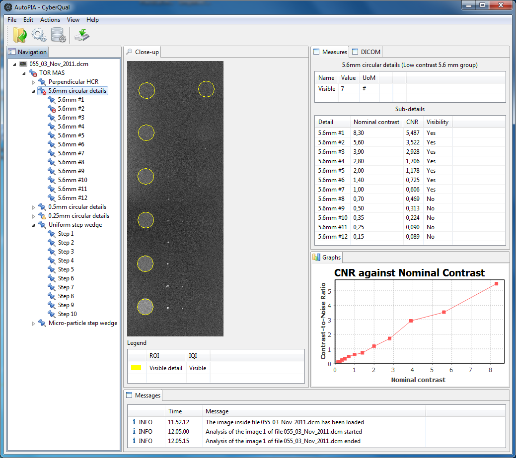
The first table of the Measures view shows the count of visible details (IQI name is visible), while the second table lists the IQIs and physical properties of all the children: in this example CNR, Visibility and Nominal Contrast.

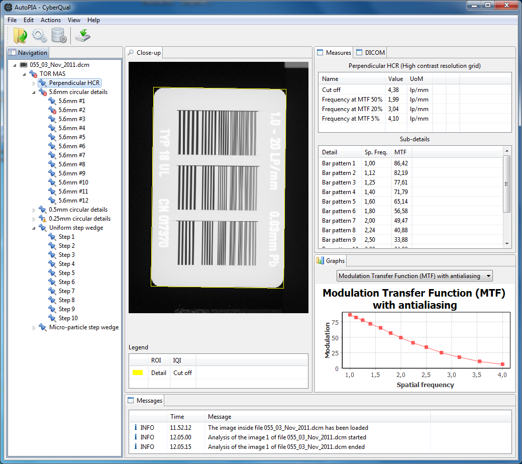
In the analysis workbench there is also the Graphs view which collects all graphs related to the selected node: for the "5.6mm circular details" the CNR against the nominal contrast. Another interestingexample is related to the detail "Perpendicular HCR" which show the Modulation Transfer Function (MTF), which has a nice graph representation.

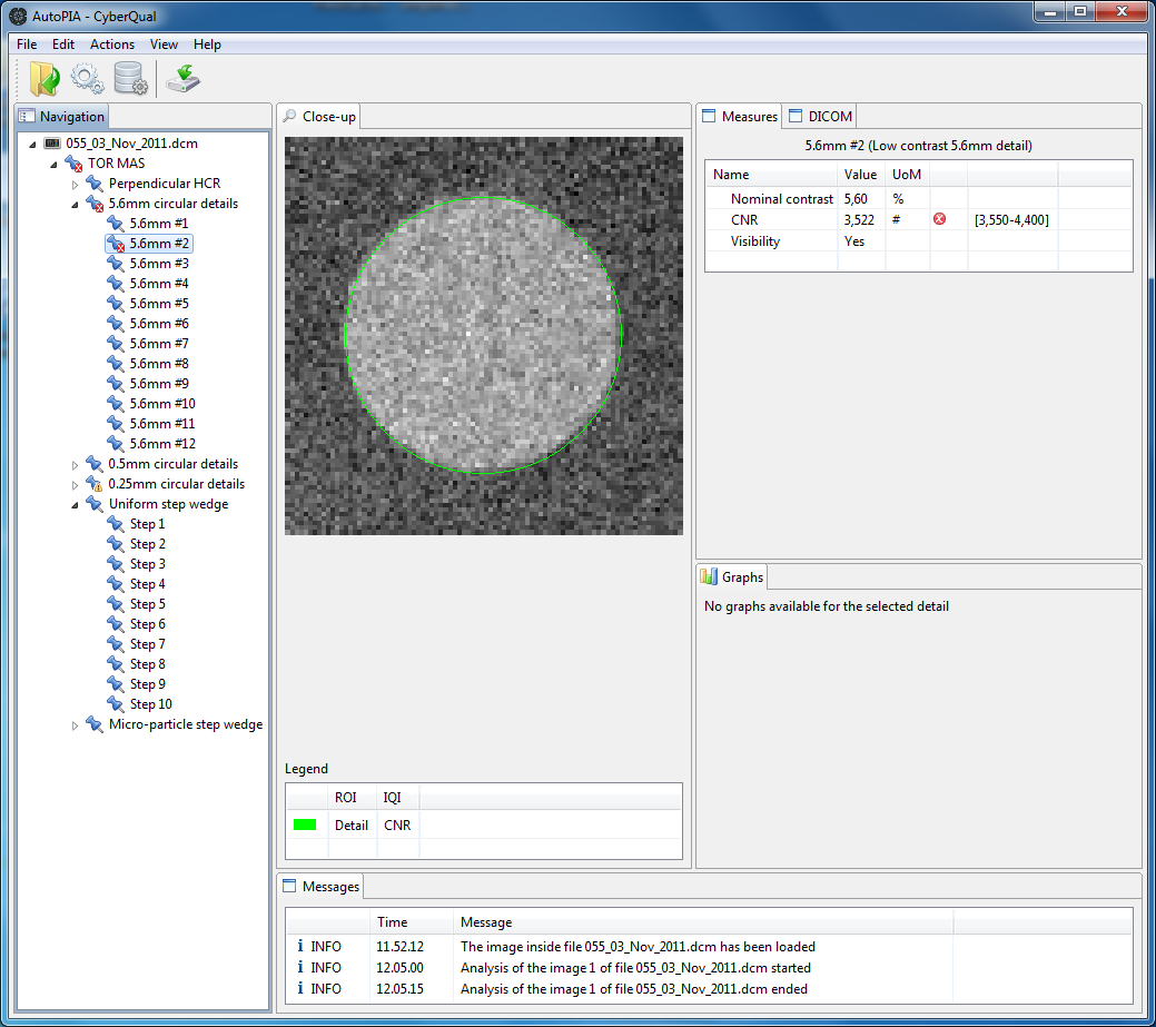
Good observers may have noticed there are markers on some nodes: they indicate that IQI values have exceeded the bounduaries set in the definition of the baseline (red marks for control bounduaries and yellow marks for warning bounduaries). When the selected node exceeds some limits, the Measures view shows which are the bounduaries, so to provide an immediate idea of what is outside the limits and for how much. Select the node "5.6mm #2" to see an example.

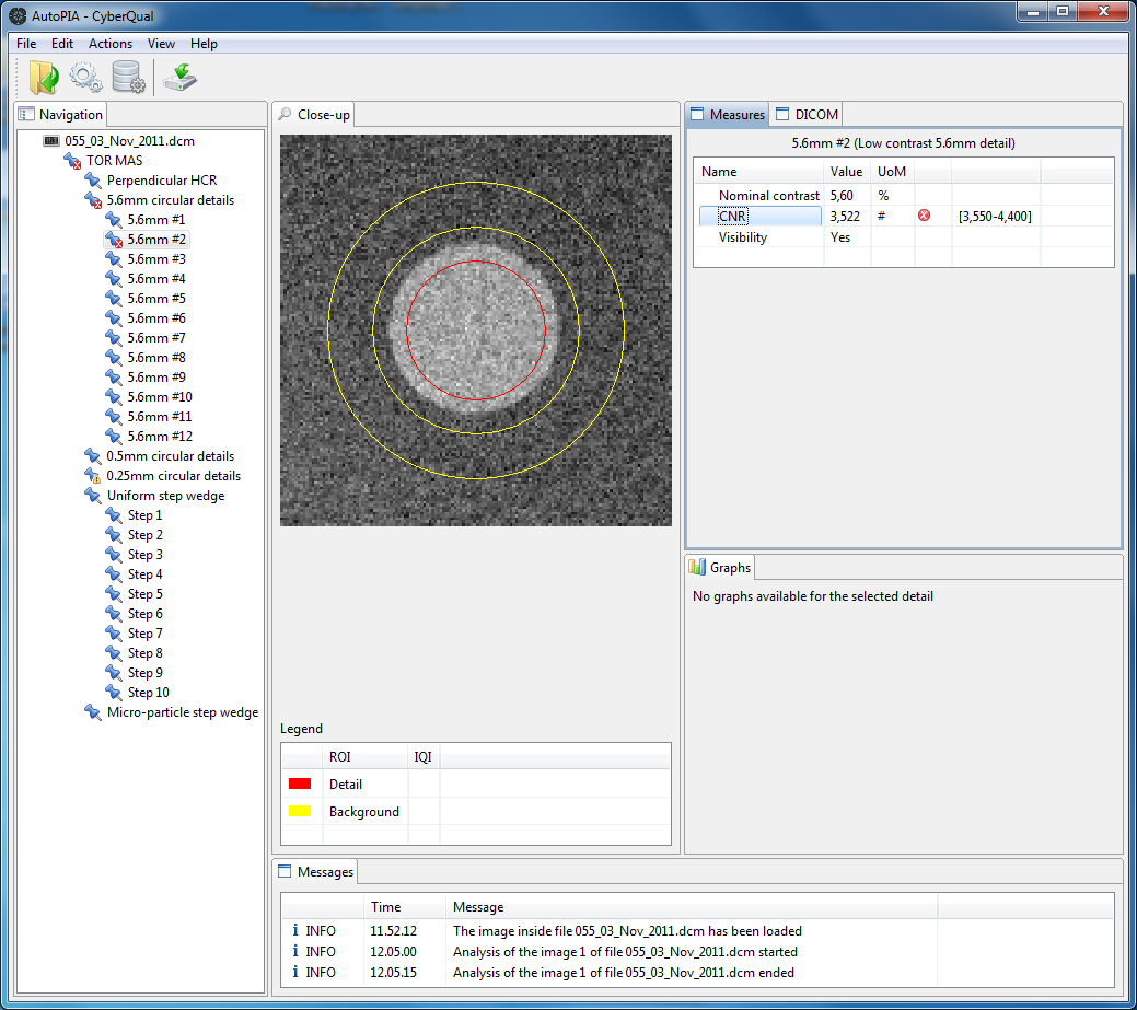
Sometimes it is very interesting and useful to understand how the IQI has been calculated; software documentation can give the formula or algorithm for the calculation, but the choice of the Regions Of Interest (ROIs) has a huge impact on the IQI value. Therfore, it is of primary importance to understand how the software choose the ROIs to calculate the IQI value. At least to have a visual confirmation that the choice is reasonable. With AutoPIA this is a very easy task: it is sufficient to select the IQI from the Measures view and the ROIs used to calculate the IQI value will be highlighted inside the Close-up view. Click on "CNR" to see the detail and background ROIs used to calculate the CNR value of the selected detail.

Let's continue with the simulation of the routine quality control: after the image analysis, it is possible to store the results and append them into the control charts. The required information include the equipment used and the date when the image has been taken. AutoPIA digs inside the image DICOM headers and reads all the necessary information from there. This is to avoid error prone and time consuming manual data entry. Therefore, clicking on the menu Actions | Store opens a dialog that has all required fields already filled, and the user has just to click on "Ok". Sometimes, the image DICOM headers are not complete: only in this rare occasions the user shall enter the information manually.

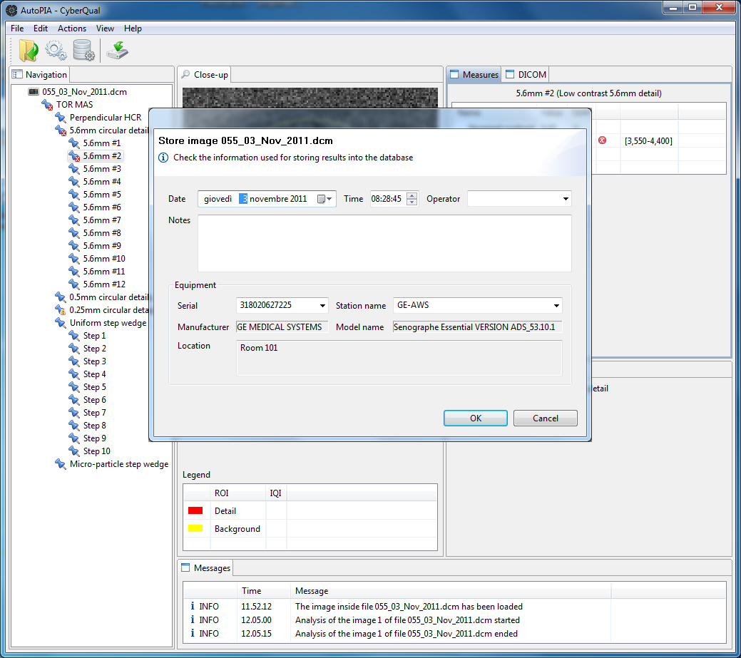
In this example, AutoPIA retrieves from the DICOM headers the serial number and date image date: the user just clicks on "Ok" and the analysis data is stored on the database and control charts are updated. Switch to the Control Chart view (menu View | Result layout) in order to see the results. Note that even here some markers have been added.

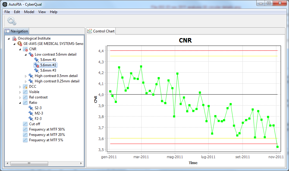
Selecting the leaf nodes with the marker will show its control charts where the graphcila representation of IQI values against baseline bounduaries immediately highlights what is going on. In this example click on "5.6mm #2" under the "CNR" IQI and you will see the IQI value taht is lower than the control bounduary.

The markers are relative only to the last image in the control chart and not to the whole period. Just to make another example, download the image 069_GE_Essential_27_Oct_2010.dcm, analyse and store it. This image has no values outside the bounduaries, therefore, all the nodes of the tree inside the Navigation view will have no markers.